Workflow • mpwR

Introduction

This vignette is a workflow template for data import and downstream analysis with mpwR including highlighting number of identifications, data completeness, quantitative and retention time precision etc. It demonstrates significant steps and showcases functions and applicability.

Loading R packages

library(mpwR)
library(flowTraceR)
library(magrittr)
library(dplyr)
library(tidyr)
library(stringr)
library(tibble)
library(ggplot2)
library(flextable)

Import

Import your data

Importing the output files from each software can be performed with prepare_mpwR. Please put all output files in one folder and follow the guidelines for naming the files. No other files/subfolders are allowed. Details are provided in the vignette Import.

files <- prepare_mpwR(path = "Path_to_Folder_with_files")

Examples

Some examples are provided to explore the workflow with create_example.

files <- create_example()

Number of Identifications

Report

The number of identifications can be determined with get_ID_Report.

ID_Reports <- get_ID_Report(input_list = files)

For each analysis an ID Report is generated and stored in a list. Each ID Report entry can be easily accessed:

flextable::flextable(ID_Reports[["DIA-NN"]])

Analysis	Run	ProteinGroup.IDs	Protein.IDs	Peptide.IDs	Precursor.IDs
DIA-NN	R01	5	5	5	5
DIA-NN	R02	5	5	5	5

Plot

Individual

Each ID Report can be plotted with plot_ID_barplot from precursor- to proteingroup-level. The generated barplots are stored in a list.

ID_Barplots <- plot_ID_barplot(input_list = ID_Reports, level = "ProteinGroup.IDs")

The individual barplots can be easily accessed:

ID_Barplots[["DIA-NN"]]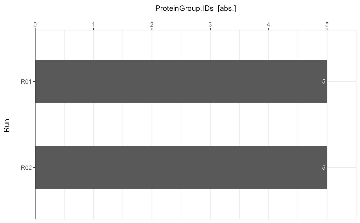

Summary

As a visual summary a boxplot can be generated with plot_ID_boxplot.

plot_ID_boxplot(input_list = ID_Reports, level = "ProteinGroup.IDs")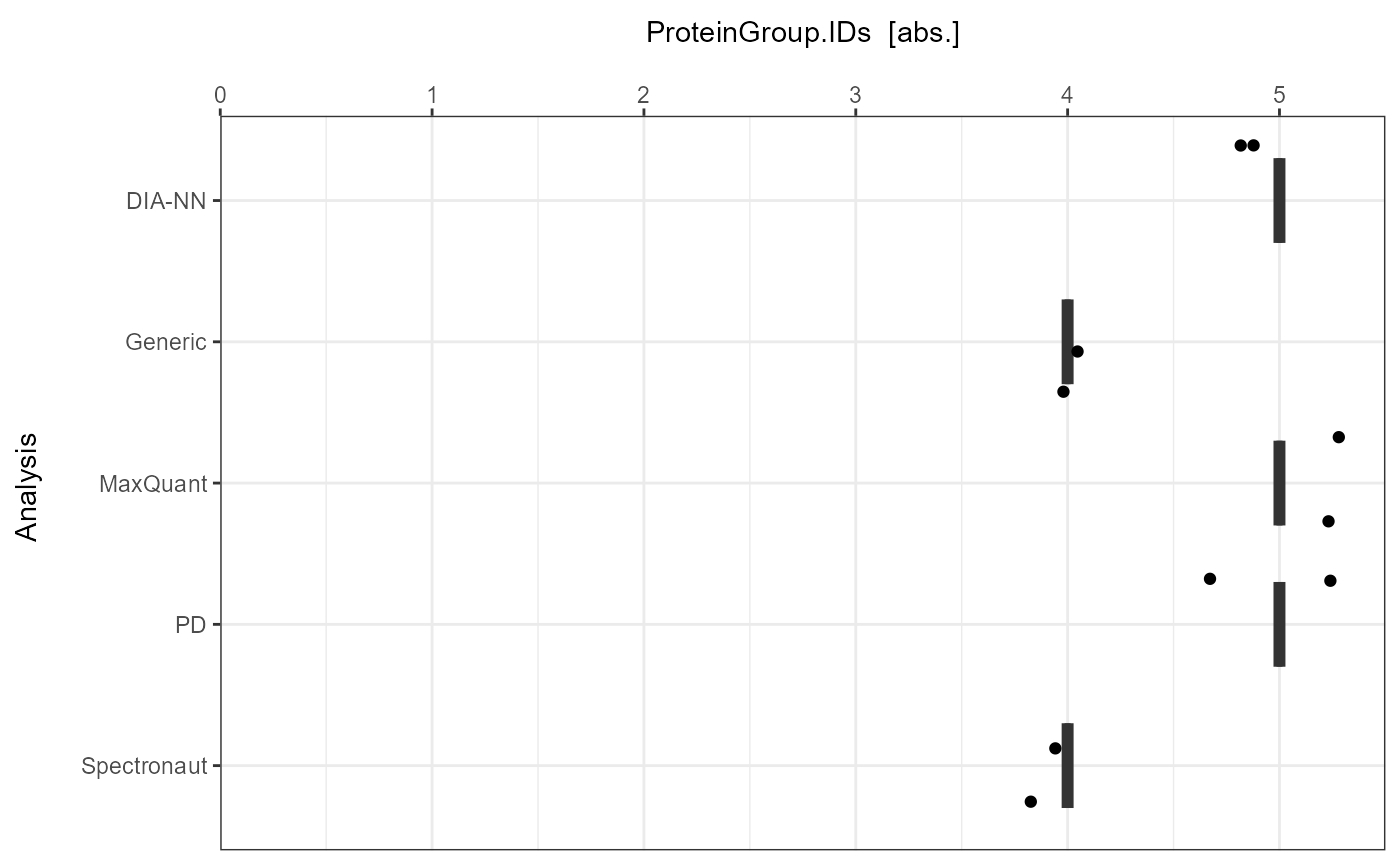

Data Completeness

Report

Data Completeness can be determined with get_DC_Report for absolute numbers or in percentage.

DC_Reports <- get_DC_Report(input_list = files, metric = "absolute")
DC_Reports_perc <- get_DC_Report(input_list = files, metric = "percentage")

For each analysis a DC Report is generated and stored in a list. Each DC Report entry can be easily accessed:

flextable::flextable(DC_Reports[["DIA-NN"]])

Analysis	Nr.Missing.Values	Precursor.IDs	Peptide.IDs	Protein.IDs	ProteinGroup.IDs	Profile
DIA-NN	1	0	0	4	2	unique
DIA-NN	0	5	5	3	4	complete

Plot

Individual

Absolute

Each DC Report can be plotted with plot_DC_barplot from precursor- to proteingroup-level. The generated barplots are stored in a list.

DC_Barplots <- plot_DC_barplot(input_list = DC_Reports, level = "ProteinGroup.IDs", label = "absolute")

The individual barplots can be easily accessed:

DC_Barplots[["DIA-NN"]]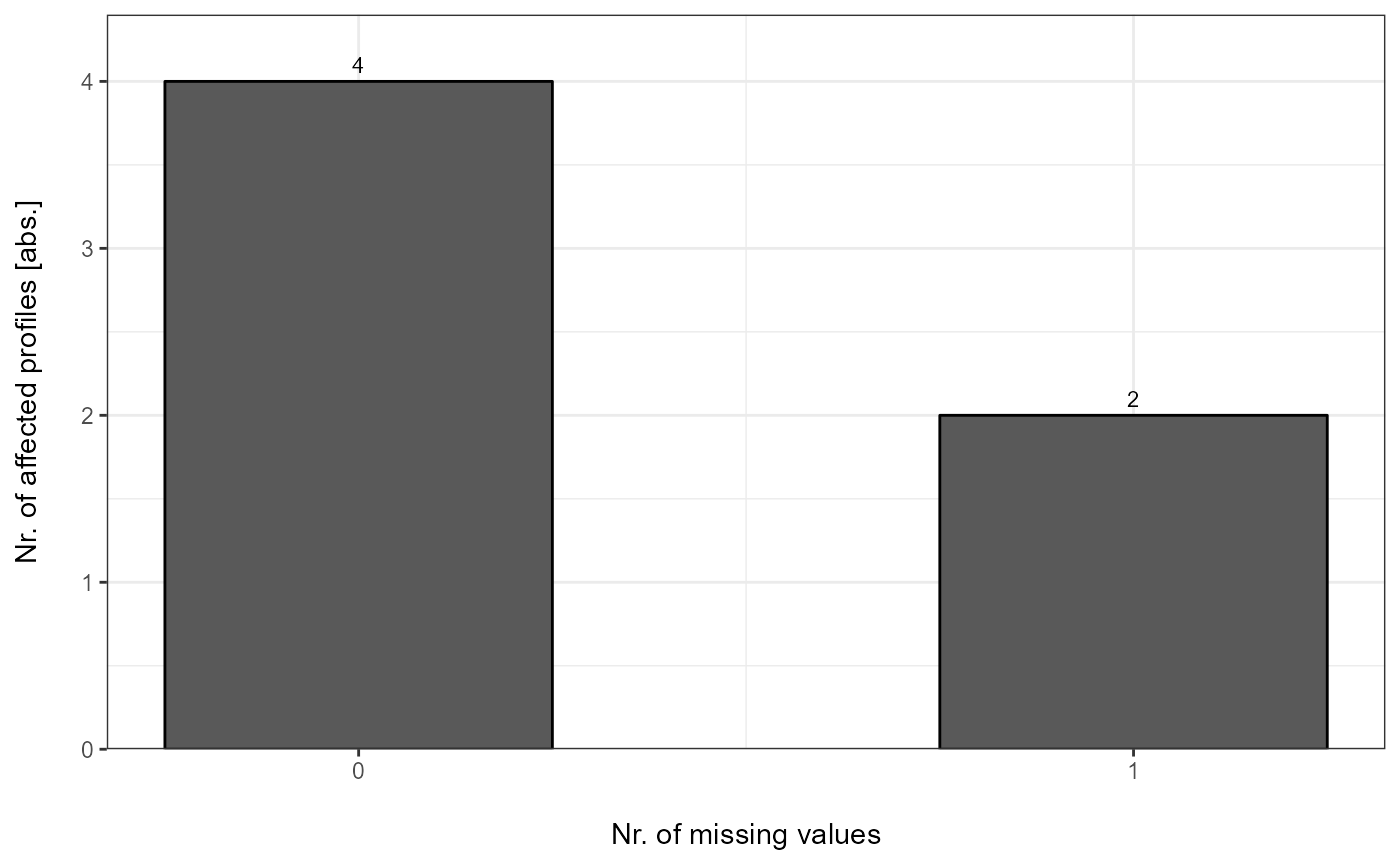

Percentage

plot_DC_barplot(input_list = DC_Reports_perc, level = "ProteinGroup.IDs", label = "percentage")[["DIA-NN"]]

Summary

As a visual summary a stacked barplot can be generated with plot_DC_stacked_barplot.

Absolute

plot_DC_stacked_barplot(input_list = DC_Reports, level = "ProteinGroup.IDs", label = "absolute")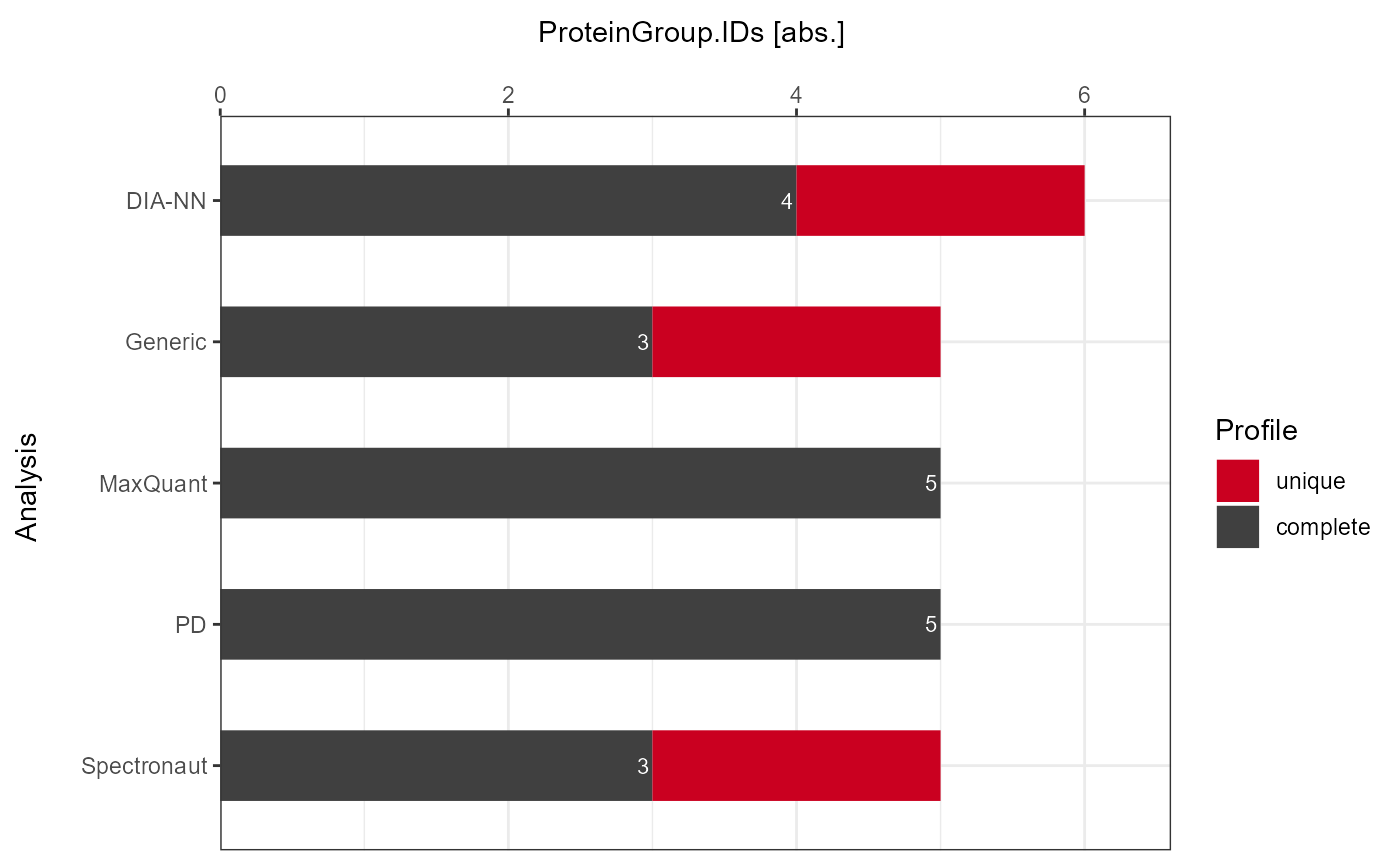

Percentage

plot_DC_stacked_barplot(input_list = DC_Reports_perc, level = "ProteinGroup.IDs", label = "percentage")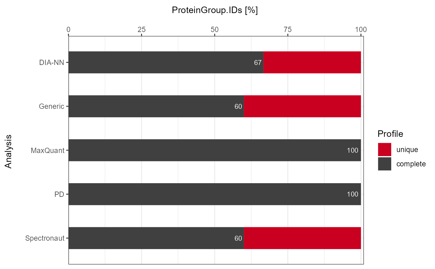

Missed Cleavages

Report

A report for Missed Cleavages can be generated with get_MC_Report for absolute numbers or in percentage.

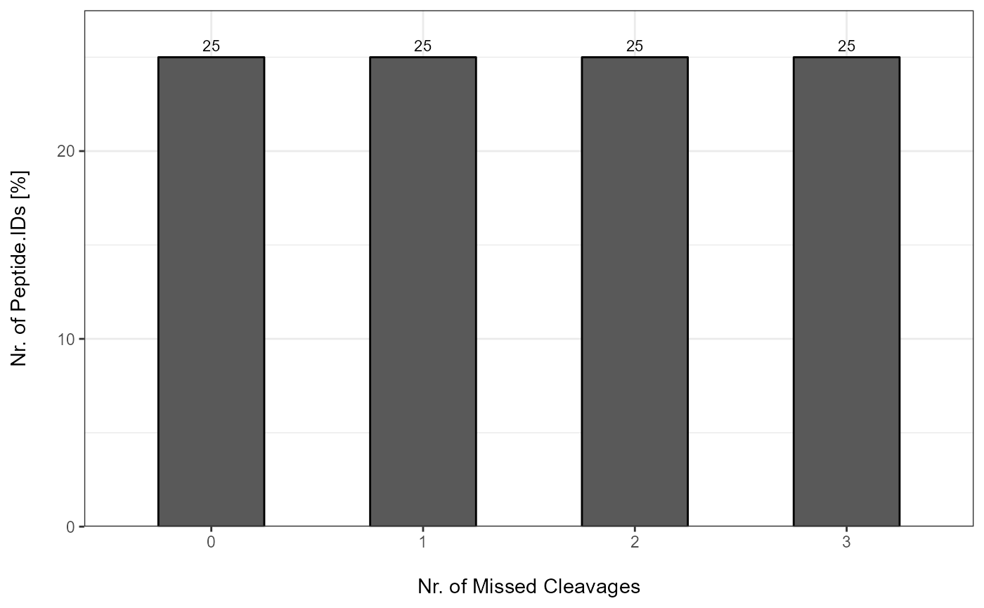
MC_Reports <- get_MC_Report(input_list = files, metric = "absolute")
MC_Reports_perc <- get_MC_Report(input_list = files, metric = "percentage")

For each analysis a MC Report is generated and stored in a list. Each MC Report entry can be easily accessed:

flextable::flextable(MC_Reports[["Spectronaut"]])

Analysis	Missed.Cleavage	mc_count
Spectronaut	0	1
Spectronaut	1	1
Spectronaut	2	1
Spectronaut	3	1

Plot

Individual

Absolute

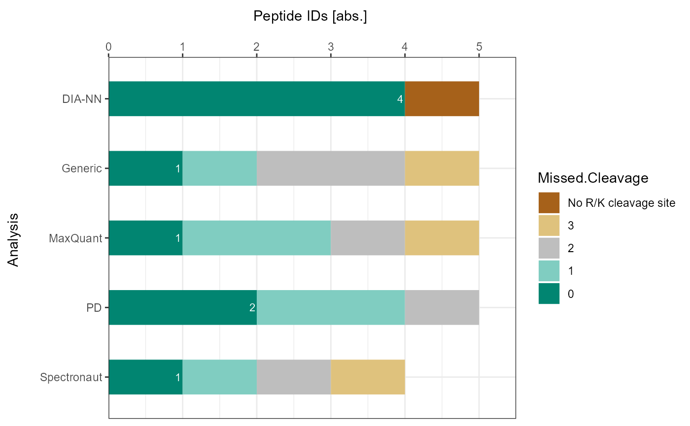
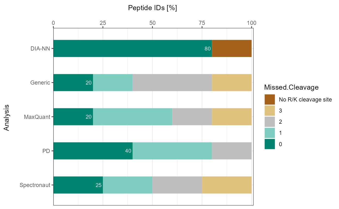
Each MC Report can be plotted with plot_MC_barplot from precursor- to proteingroup-level. The generated barplots are stored in a list.

MC_Barplots <- plot_MC_barplot(input_list = MC_Reports, label = "absolute")

The individual barplots can be easily accessed:

MC_Barplots[["Spectronaut"]]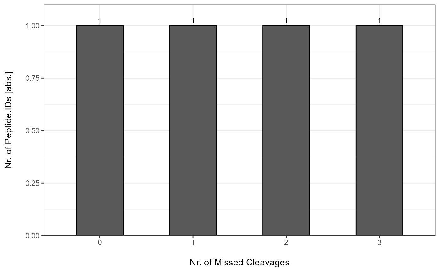

Percentage

plot_MC_barplot(input_list = MC_Reports_perc, label = "percentage")[["Spectronaut"]]

Summary

As a visual summary a stacked barplot can be generated with plot_MC_stacked_barplot.

Absolute

plot_MC_stacked_barplot(input_list = MC_Reports, label = "absolute")

Percentage

plot_MC_stacked_barplot(input_list = MC_Reports_perc, label = "percentage")

Retention Time Precision

Preparation

The coefficient of variation (CV) can be calculated with get_CV_RT. Only complete profiles are used.

CV_RT <- get_CV_RT(input_list = files)

Plot

As a visual summary a density plot for all analyses can be accessed via plot_CV_density.

plot_CV_density(input_list = CV_RT, cv_col = "RT")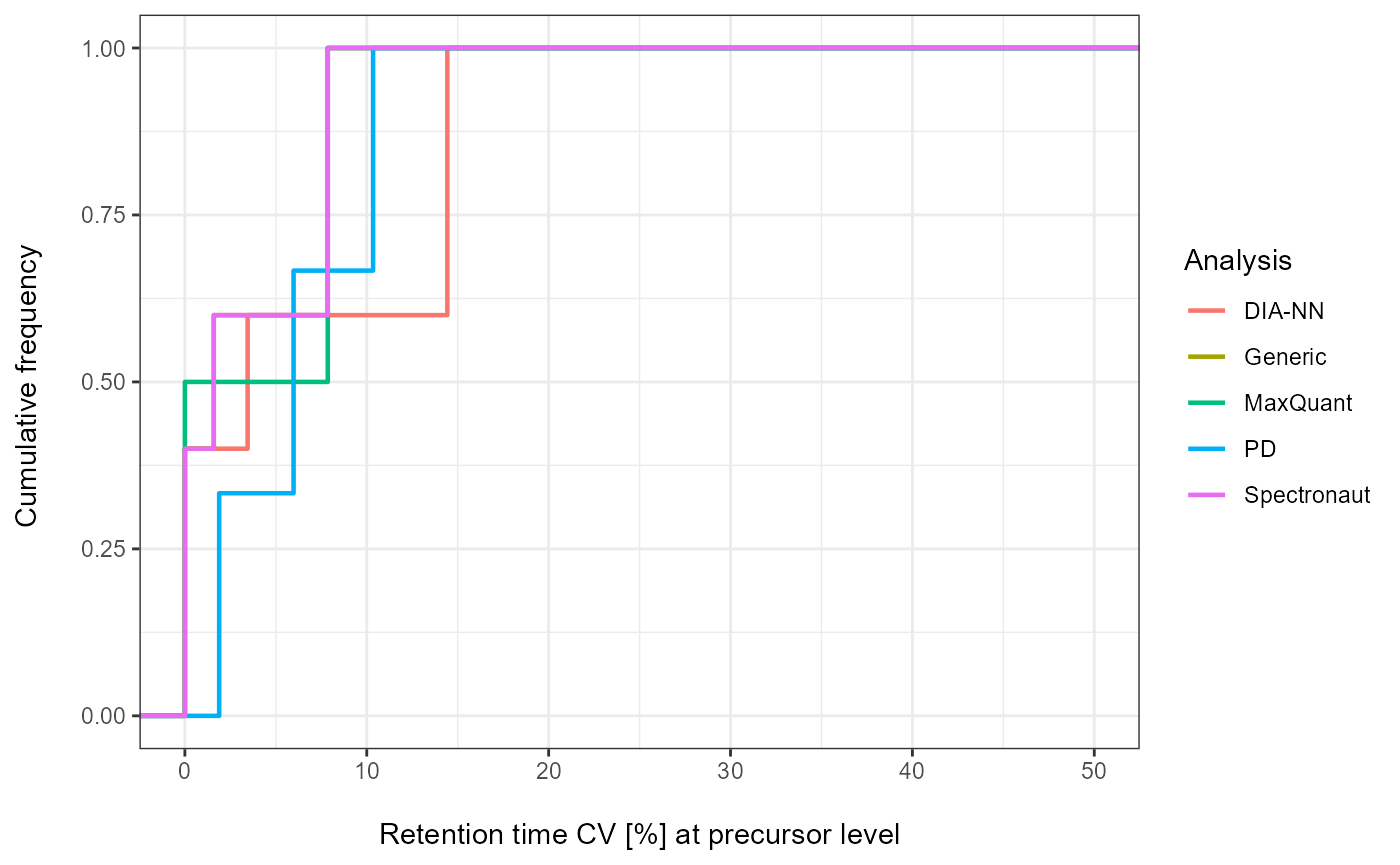

Quantitative Precision

Peptide-level

Preparation

The CV can be calculated with get_CV_LFQ_pep. Only complete profiles are used.

CV_LFQ_Pep <- get_CV_LFQ_pep(input_list = files)
#> For DIA-NN no quantitative LFQ data on peptide-level.
#> For PD no quantitative LFQ data on peptide-level.

Plot

As a visual summary a density plot for all analyses can be accessed via plot_CV_density.

plot_CV_density(input_list = CV_LFQ_Pep, cv_col = "Pep_quant")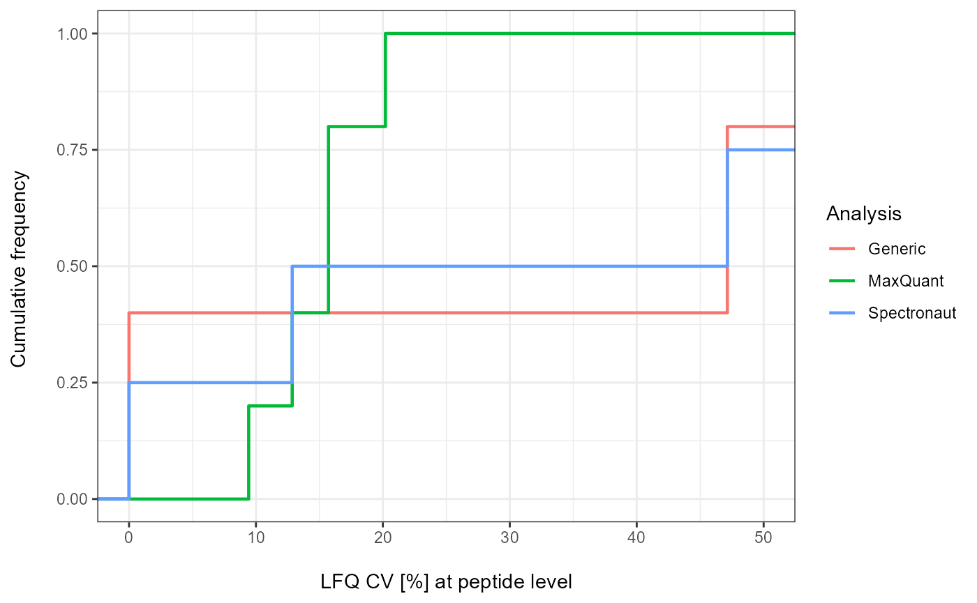

Proteingroup-level

Preparation

The CV can be calculated with get_CV_LFQ_pg. Only complete profiles are used.

CV_LFQ_PG <- get_CV_LFQ_pg(input_list = files)
#> For PD no quantitative LFQ data on proteingroup-level.

Plot

As a visual summary a density plot for all analyses can be accessed via plot_CV_density.

plot_CV_density(input_list = CV_LFQ_PG, cv_col = "PG_quant")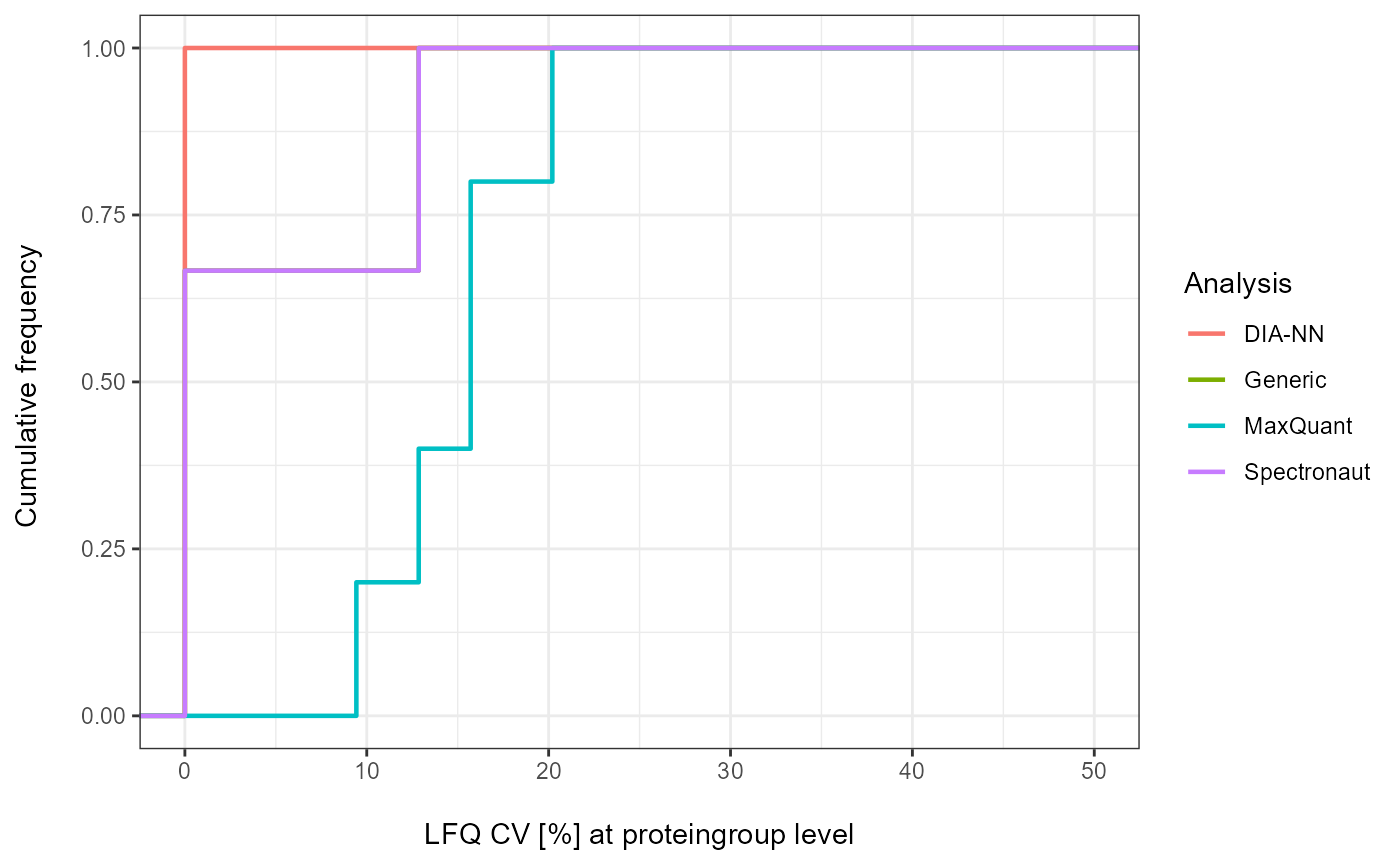

Upset Plot

Common identifications and intersections between analyses can be highlighted.

Preparation

Use get_Upset_list to prepare for Upset plotting.

Upset_prepared <- get_Upset_list(input_list = files, level = "ProteinGroup.IDs")

Plot

The Upset plot can be generated with plot_Upset.

plot_Upset(input_list = Upset_prepared, label = "ProteinGroup.IDs")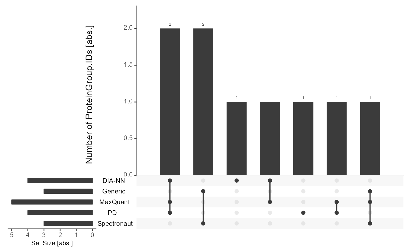

Inter-software Comparison - flowTraceR

Functions of the package flowTraceR are incorporated in mpwR for inter-software comparisons. Software outputs are standardized and easily comparable.

Precursor-level without flowTraceR

Without standardizing the precursor-level information, the software outputs only form software-dependent cluster.

get_Upset_list(input_list = files, level = "Peptide.IDs") %>% #prepare Upset
  plot_Upset(label = "Peptide.IDs") #plot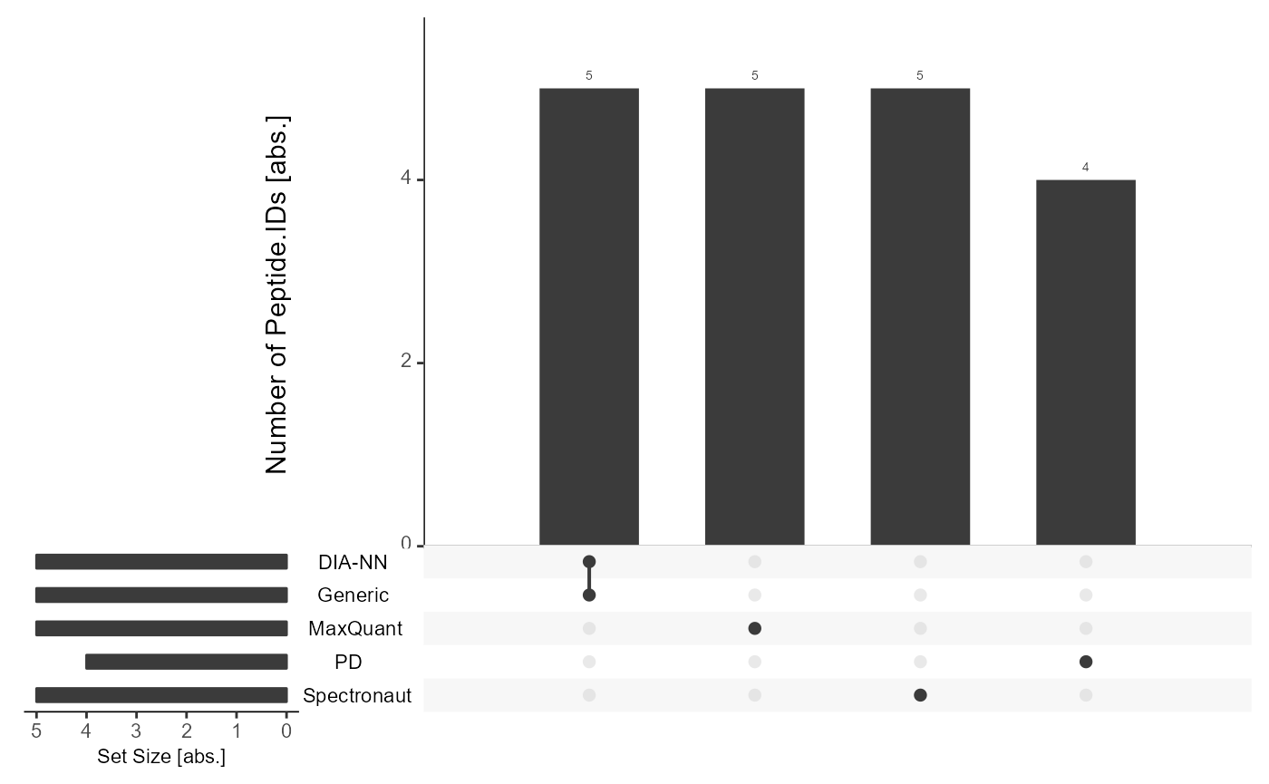

Precursor-level with flowTraceR

By enabling flowTraceR the precursor-level information is standardized and common identifications can be inferred.

get_Upset_list(input_list = files, level = "Peptide.IDs", flowTraceR = TRUE) %>% #prepare Upset
  plot_Upset(label = "Peptide.IDs") #plot
#> flowTraceR not available for generic input. No conversion applied for position 5 in input_list.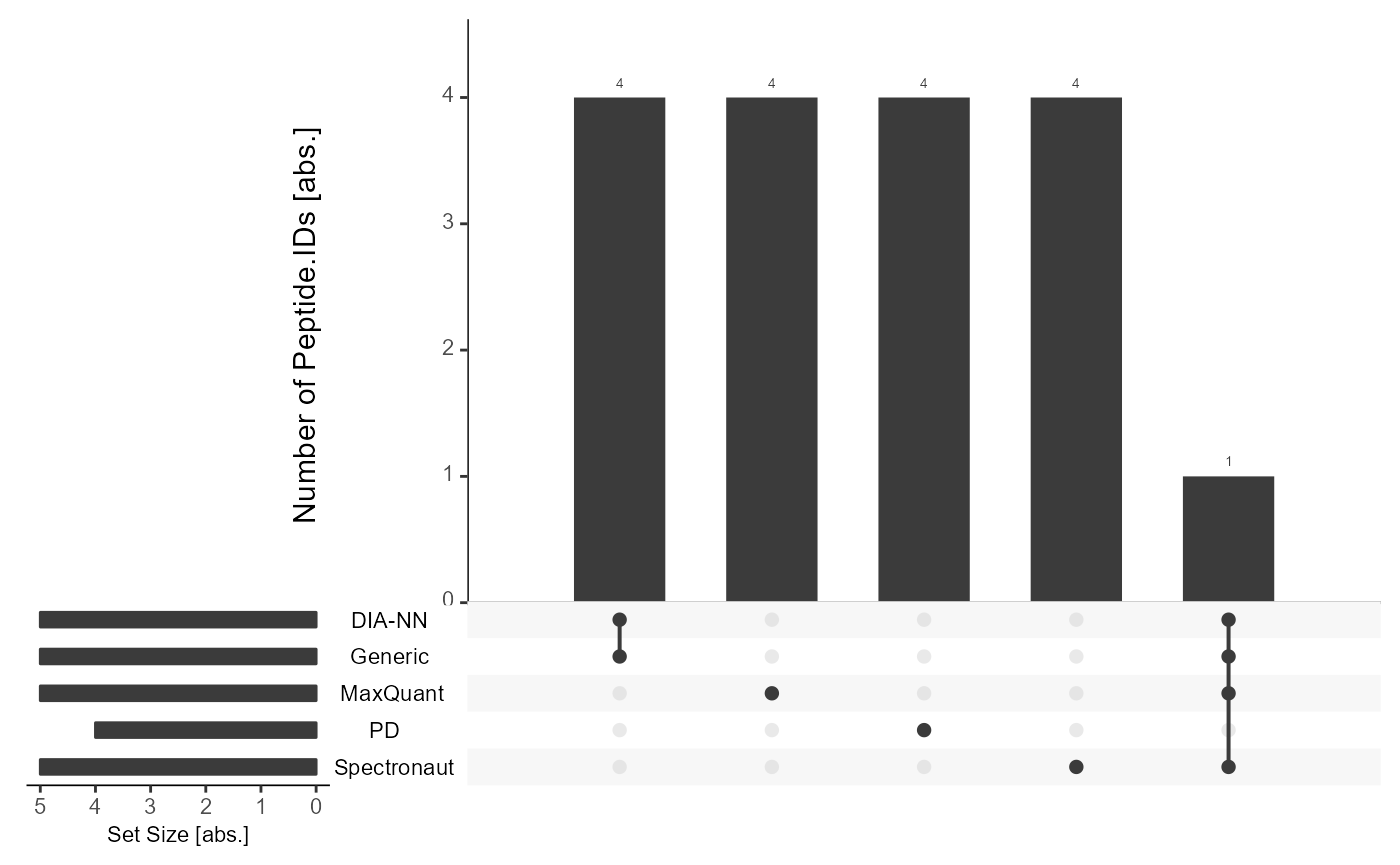

Summary

mpwR offers functions to summarize the downstream analysis.

Report

A summary report can be generated with get_summary_Report.

Summary_Report <- get_summary_Report(input_list = files)

Plot

As a visual summary a radar chart for all analyses can be accessed via plot_radarchart.

Overview

plot_radarchart(input_df = Summary_Report)

Details

To highlight individual categories, the generated summary report can be easily adjusted and used for plotting.

#Focus on Data Completeness
Summary_Report %>%
  dplyr::select(Analysis, contains("Full")) %>% #Analysis column and at least one category column is required
  plot_radarchart()